Enhanced Sentinel 2 Agriculture

1. Introduction

Land management and, in particular, management of cultivated land plays a central role globally to sustain economic growth, and will play an ever-important role in reducing the impact of climate change.

Earth Observations (EO) information is particularly suited for land management applications, as it provides global coverage at high spatial resolution and high revisit frequency. In particular, data from the Sentinel-2 satellites, freely available through the Copernicus programme, have opened up new and unique opportunities.

This challenge aims at exploring novel Artificial Intelligence (AI) methods to push the limits of Sentinel-2 time-series beyond its 10-meter pixel resolution. In particular, the challenge will focus on cultivated land, given its paramount importance for sustainable food security and global subsistence.

2. Aim of the Challenge

The aim of this challenge is to create AI methods that can exploit the temporal information of Sentinel-2 images to artificially enhance its spatial resolution, i.e. the physical size of a pixel in an image.

Your task will be to estimate a cultivated land binary map at 2.5 metres spatial resolution given as input a Sentinel-2 time-series at 10 metres spatial resolution, therefore resulting in a 4x spatial resolution enhancement.

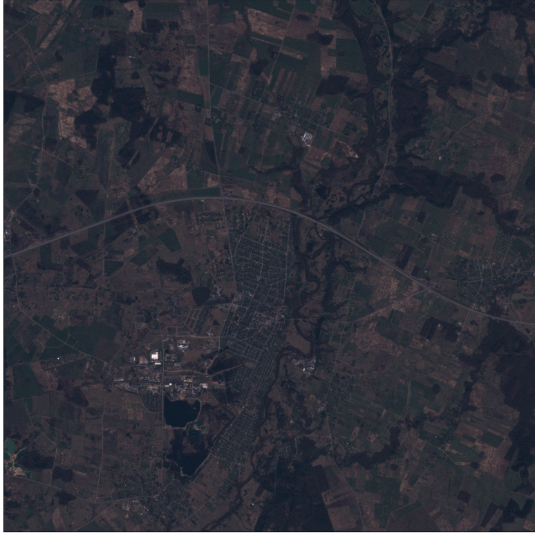
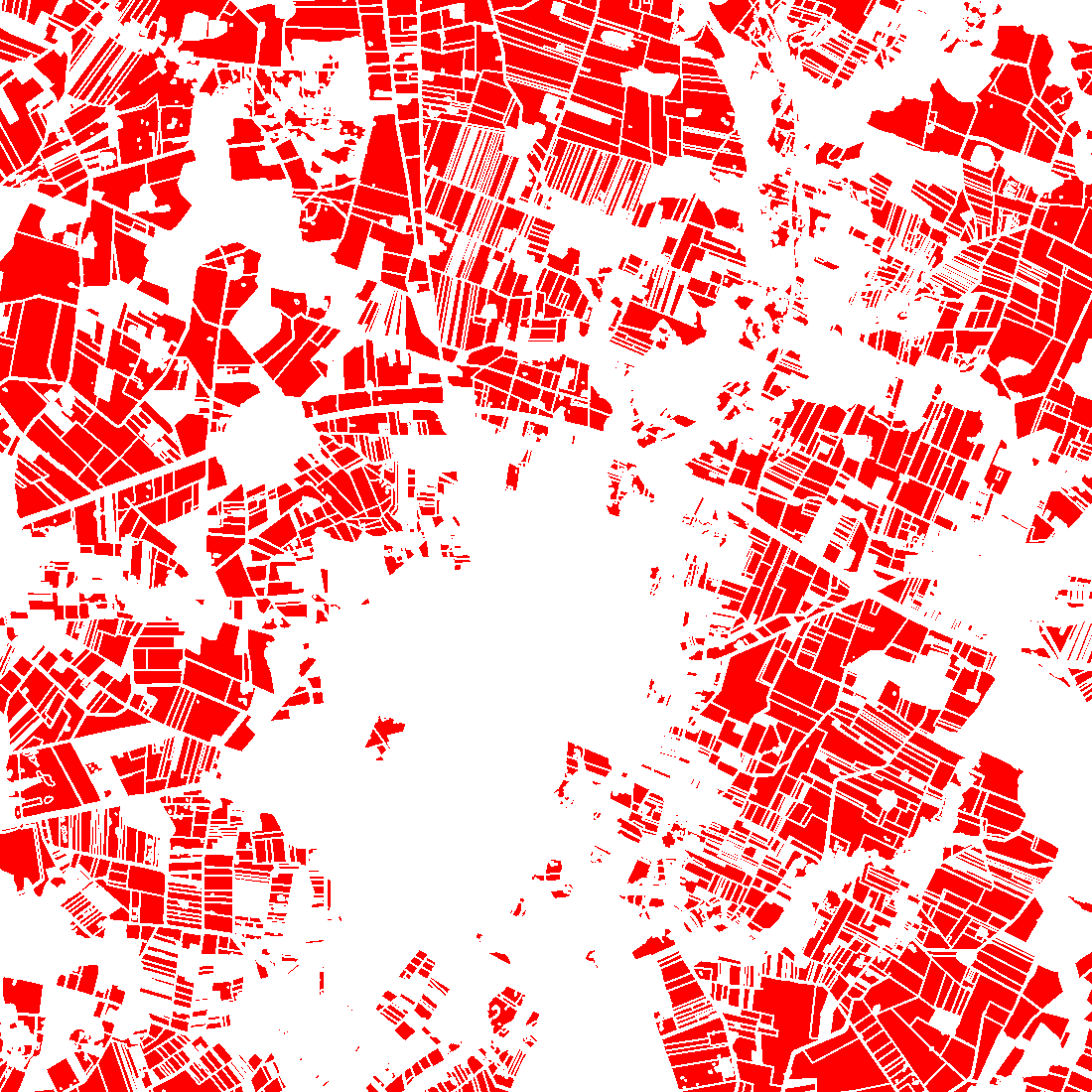
Example of Sentinel-2 time-series at 10m spatial resolution (left), and predicted cultivated land map at 2.5m spatial resolution (right).

Inspired by recent advances in AI methods for super-resolution, you will create novel end-to-end methods to model complex spatio-temporal dependencies, and extract invaluable land management information at the sub-pixel level. Such methods have the potential to revolutionize the applications of Sentinel-2 (and similar) imagery.

The inputs and outputs of the challenge can be summarised as follows:

• Inputs:
  • Sentinel-2 MSI time-series at 10m for a growing season:
    • 1st March - 1st September 2019;
    • Bottom-of-Atmosphere L2A products;
    • 12 multi-spectral bands (20m and 60m interpolated to 10m), scene classification, cloud masks.
• Outputs:
  • Cultivated land binary mask at 2.5m.

3. Areas of Interest

The area-of-interest (AOI) chosen for this challenge is the Republic of Slovenia and its neighbouring countries.

The AOI is split into 125 bounding boxes across the entire area. Data for 100 bounding boxes will be used for training only, while the remaining 25 bounding boxes will be used for computing your validation ranking. Each bounding box has a 5km x 5km size, resulting in a 500 x 500 pixel Sentinel-2 time-series, and a 2000 x 2000 pixel cultivated land map.

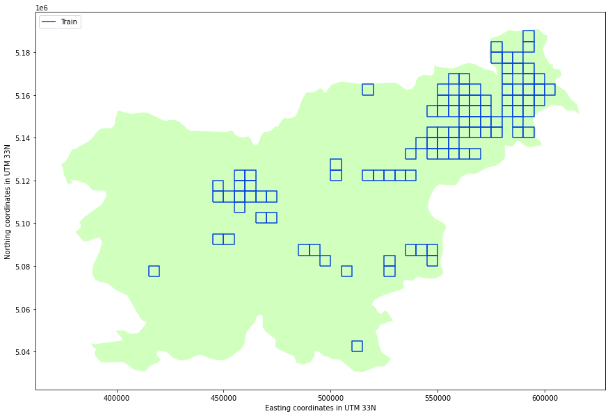
Distribution of the 100 train bounding boxes over the AOI.

4. Metrics

As is common in AI challenges, the training dataset provided includes reference labels, to be used to train and evaluate your algorithm. To test and validate your model, we provide a testing dataset consisting of 25 bounding boxes sampled from the same area. The testing dataset contains only the imaging information, and will be used to evaluate your algorithm against other teams.

To evaluate your model, you will submit the estimated cultivated land binary mask for the 25 test bounding boxes at the target 2.5m spatial resolution. The submission will be evaluated by computing the weighted Matthews Correlation Coefficient between the reference map and your models' estimates as follows:

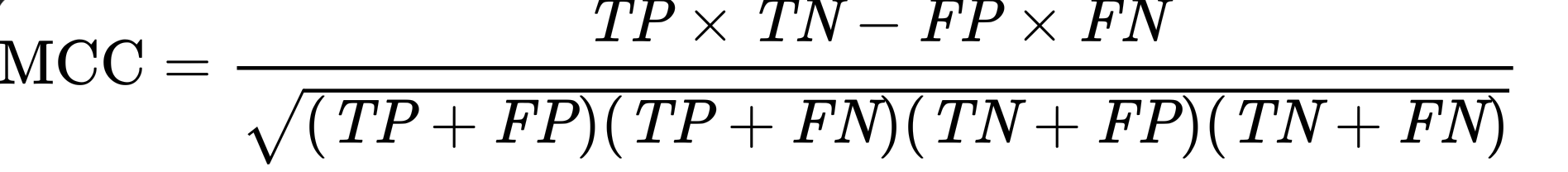
where TP, TN, FP and FN respectively denote true positives, true negatives, false positives and false negatives. This metric is particularly suited to evaluate binary classification outcomes with a very unbalanced class label distribution (as is the case for the cultivated land map where there are many more 0s than 1s). The MCC scores range from -1 (perfect mismatch with reference labels) to 1 (perfect match with reference labels).

The weighting scheme gives more weight, e.g. relevance, to small parcels, and to the contouring background that singles them out. Ideally, your algorithm should be able to classify and recover all single cultivated parcels, in particular the smaller ones since they are the most challenging. A weight is assigned to each pixel according to its cultivated/not-cultivated label, and to the size of the cultivated parcel, following a skewed normal distribution.

Code to derive such weight map is provided in the starter-pack notebook, so that the same evaluation criteria as the one used for the leaderboard ranking can be used to optimise your algorithm.

5. Leaderboard formation

Submitted entries will be ranked based on the MCC score as outlined above. Higher scores denote better estimation of the reference data, and will result in a better rank position.

To reduce the effect of over-fitting to the test dataset, as is common in AI challenges, a public and a private subset of locations are extracted from the 25 test bounding boxes. The public locations will be used to rank submission during the duration of the competition, while the private locations will be used to compute the final ranking used to crown the winners. When challenge closes, we recompute the ranking based on the private score rather than the public. This might lead to slight differences in ranking positions, since the score on the private subset might slightly differ from the public subset.

As outlined in the challenge rules, the leaderboard ranking will be combined with a qualitative evaluation from a jury, with a 0.75 and 0.25 weighting factor respectively. Check the challenge rules for details about the criteria used by the jury to assess your AI system and about the reproducibility of your submitted entries.

6. Get started

To get you started with the challenge, we have created a Jupyter notebook to guide through data download, data analysis and an example of a valid submission.

Find the starter-pack including the Jupyter notebook and the required utility and metadata files in this GitHub repository.

Alongside the starter-pack, for this challenge we are happy to provide you with free computational resources, made available through the Euro Data Cube (EDC). Read on to find out how to access these resources, or how to download the data.

6.1. Computational resources

Whether you are using EDC or your own computational resources, you will be provided with a Docker image setting up a Python environment that includes a large collection of geospatial libraries (e.g. rasterio to process image data, shapely to process vector data, geopandas to process structured geospatial data, eo-learn to build processing pipelines of spatio-temporal data) and machine learning libraries (e.g. scikit-learn, ligthgbm, PyTorch, TensorFlow) libraries.

You are required to use the provided Python environment, as it provides the same starting point to all participants. However, you are allowed add to the environment public Python libraries that are not included, as long as the jury can reproduce the installation, e.g. by including !pip install public-library in your code.

6.1.1 Euro Data Cube resources

Free computational resources are made available to participants that require so. If you don't have access to a GPU for training of your methods, GPU-powered instances are made available through the EDC EOxHub Workspace.

To require EDC resources sign-up to EDC through this link.

Once you will sign-up to EDC, follow the instructions to get access to your hosted workspace. It can take from few hours to few working days to get access to the resources.

The hosted workspace will be already configured with the APIs required to download the data. The starter-pack content will be mounted as a read-only folder named s3. Upon activation of your account, access your Jupyter-Lab environment via link available on your dashboard.

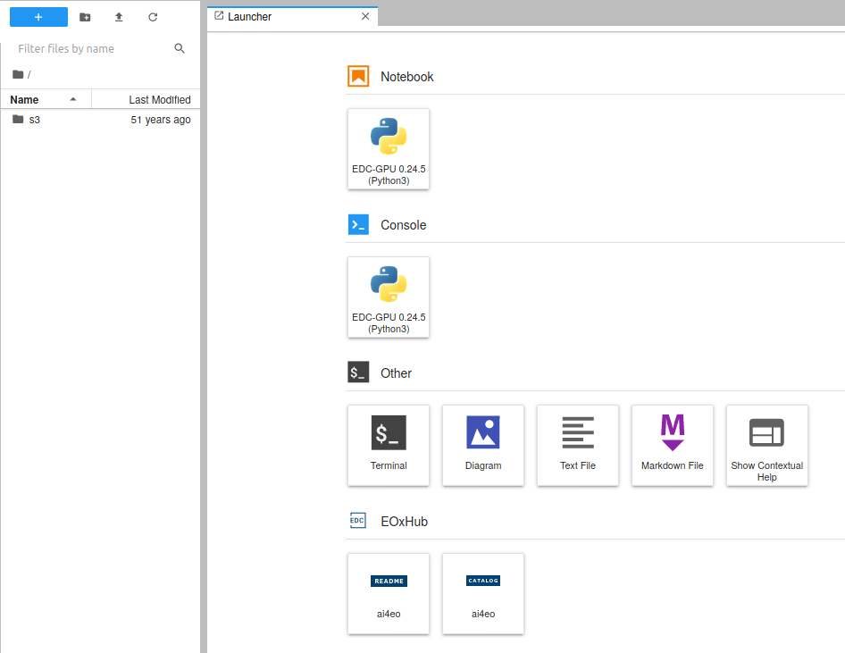
Jupyter-Lab hosted workspace.

Select the ai4eo README at bottom left of your EOxHub Section, open the linked starter-pack notebook and click on Execute Notebook at the top left. Copy the file to the home directory of your workspace. You are now ready to run the notebook.

6.1.2 Personal resources

The following instructions will help you set-up the Docker environment from which you can develop your solution. The following instruction apply to Linux-based operating systems.

Download from the EDC GitHub repository the DockerFile and build the image by executing from your terminal

git clone https://github.com/eurodatacube/base-images.git
cd base-images
docker build -f Dockerfile-jupyter-user-g -t ai4eo .

You should see the built image by running docker images. Take a note of the IMAGE ID.

If you have access to an NVIDIA GPU with CUDA set-up, you need to install nvidia-docker as follows

#setup distribution for nvidia-container
curl -s -L https://nvidia.github.io/nvidia-container-runtime/gpgkey | \
  sudo apt-key add -
distribution=$(. /etc/os-release;echo $ID$VERSION_ID)
curl -s -L https://nvidia.github.io/nvidia-container-runtime/$distribution/nvidia-container-runtime.list | \
  sudo tee /etc/apt/sources.list.d/nvidia-container-runtime.list
sudo apt-get update

#install
apt-get install nvidia-container-runtime
apt-get install nvidia-docker2

#restart daemon
sudo systemctl restart docker

Depending on your Docker version, you can access the environment running one of the following commands (if you don't have a GPU simply run docker run -p 8888:8888 <IMAGE ID>)

# for Docker versions earlier than 19.03
docker run -p 8888:8888 --runtime nvidia <IMAGE ID>

# for Docker versions later than 19.03
docker run -p 8888:8888 --gpus all  <IMAGE ID>

The Jupyter environment should be now accessible by browsing to 127.0.0.1:8888 with your favourite web browser. You can modify the port numbers (i.e. 8888) to your personal preference, as well as add flags to give the Docker environment access to your local directories.

6.2. Data download

To get started with challenge you need training data to develop your algorithm, and testing data to submit your solution.

Given the large size of the required training dataset (~12GB on disk), we provide access to Sentinel-2 imagery and the reference cultivated land polygons through the Sentinel Hub and GeoDB web APIs, respectively. The APIs allow to download data for each of the 100 training bounding boxes separately, therefore reducing data transfer issues.

The TEST DATASET can be downloaded only through direct link available in the Download Section at the top of this page (requires sign-in).

Regardless of how you get access to the data, follow the instructions provided in the starter-pack notebook to execute checks on the correctness of the downloaded files.

6.2.1 APIs

Accounts for Sentinel Hub and GeoDB are required to download the data through their APIs. If you are using the EDC EOxHub hosted workspace, the accounts are already created and set-up for you and no further action is required. If you are using your own resource and don't have an account yet, you can quickly set-up a trial account by following the instructions provided in the starter-pack notebook.

6.2.2 Direct link

The training dataset as a .tar.gz compressed file is also available for direct download. The size of the file is 10.7GB. Consult the notebook to run file checks to confirm correctness of download. The link to the direct download of the training dataset is provided in the Download Section at the top of this page (requires sign-in).