Seeing Beyond the Visible

You are free to use and/or refer to the HYPERVIEW dataset in your own research (non-commercial use), provided that you cite the following manuscript:

[1] J. Nalepa, B. Le Saux, N. Longépé, L. Tulczyjew, M. Myller, M. Kawulok, K. Smykala; Michal Gumiela, "The Hyperview Challenge: Estimating Soil Parameters from Hyperspectral Images," 2022 IEEE International Conference on Image Processing (ICIP), 2022, pp. 4268-4272, doi: 10.1109/ICIP46576.2022.9897443. (https://ieeexplore.ieee.org/document/9897443)

[2] J. Nalepa et al., "Estimating Soil Parameters From Hyperspectral Images: A benchmark dataset and the outcome of the HYPERVIEW challenge," in IEEE Geoscience and Remote Sensing Magazine, doi: 10.1109/MGRS.2024.3394040. (https://ieeexplore.ieee.org/document/10526314)

The bibtex of [1] and [2] are:

@INPROCEEDINGS{9897443,
  author={Nalepa, Jakub and Le Saux, Bertrand and Longépé, Nicolas and Tulczyjew, Lukasz and Myller, Michal and Kawulok, Michal and Smykala, Krzysztof and Gumiela, Michal},
  booktitle={2022 IEEE International Conference on Image Processing (ICIP)},
  title={The Hyperview Challenge: Estimating Soil Parameters from Hyperspectral Images},
  year={2022},
  pages={4268-4272},
  doi={10.1109/ICIP46576.2022.9897443}
}

@ARTICLE{10526314,
  author={Nalepa, Jakub and Tulczyjew, Lukasz and Le Saux, Bertrand and Longépé, Nicolas and Ruszczak, Bogdan and Wijata, Agata M. and Smykala, Krzysztof and Myller, Michal and Kawulok, Michal and Kuzu, Ridvan Salih and Albrecht, Frauke and Arnold, Caroline and Alasawedah, Mohammad and Angeli, Suzanne and Nobileau, Delphine and Ballabeni, Achille and Lotti, Alessandro and Locarini, Alfredo and Modenini, Dario and Tortora, Paolo and Gumiela, Michal},
  journal={IEEE Geoscience and Remote Sensing Magazine},
  title={Estimating Soil Parameters From Hyperspectral Images: A benchmark dataset and the outcome of the HYPERVIEW challenge},
  year={2024},
  volume={},
  number={},
  pages={2-30},
  keywords={Soil;Satellites;Artificial intelligence;Monitoring;Vegetation mapping;Reproducibility of results;Magnesium},
  doi={10.1109/MGRS.2024.3394040}
}

Objective of the Challenge

The objective of this challenge is to automate the process of estimating the soil parameters, specifically, potassium ($K$), phosphorus pentoxide ($P_2O_5$), magnesium ($Mg$) and $pH$, through extracting them from the airborne hyperspectral images captured over agricultural areas in Poland (the exact locations are not revealed). To make the solution applicable in real-life use cases, all the parameters should be estimated as precisely as possible.

The dataset comprises 2886 patches in total (2 m GSD), of which 1732 patches for training and 1154 patches for testing. The patch size varies (depending on agricultural parcels) and is on average around 60x60 pixels. Each patch contains 150 contiguous hyperspectral bands (462-942 nm, with a spectral resolution of 3.2 nm), which reflects the spectral range of the hyperspectral imaging sensor deployed on-board Intuition-1.

The participants are given a training set of 1732 training examples. The examples are hyperspectral image patches with the corresponding ground-truth information. Each masked patch corresponds to a field of interest, as presented in Fig. 1. Ground truth are the soil parameters obtained for the soil samples collected for each field of interest in the process of laboratory analysis, and is represented by a 4-value vector.

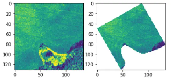
Fig. 1: The participants are given the masked hyperspectral image patches corresponding to the fields of interest (one masked patch is a single field), and should estimate the four soil parameters based on the available image data.

Given the training data, the Teams develop their solutions that will be validated over the test data, for which the target (ground-truth) parameter values are not revealed.

Metrics

The score obtained by a Team will be calculated using the following formula:

where

and $|\psi|$ denotes the cardinality of the test set.

Here, we calculate four $MSE_i$ values over the entire test set $\psi$, one for each soil parameter ($K$, $P_2O_5$, $Mg$ and $pH$), and divide them by the corresponding $MSE$ value obtained using a trivial baseline algorithm which returns the average parameter value obtained from the training set.

The lower score values denote the better solutions, with Score=0 indicating the perfect one.

Illustrative example

Let us assume the following:

1. We have three competing algorithms: Algorithm A, Algorithm B, and Algorithm C, resulting in some MSE values obtained for all parameters of interest.
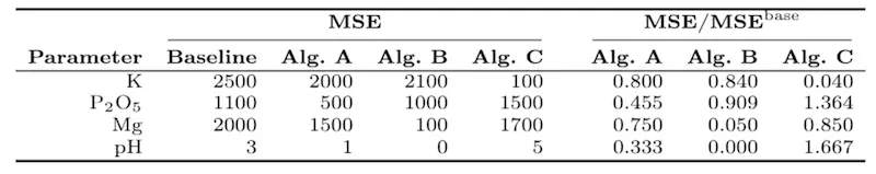
2. The trivial baseline algorithm obtains the following MSE scores (over the entire test set) for $K$, $P_2O_5$, $Mg$ and $pH$: 2500, 1100, 2000 and 3, respectively.

Then, Table 1 gathers the baseline MSE together with the MSE values obtained by the algorithms A – C, and divided by the baseline MSE. The baseline MSE reflects the performance of the algorithm that returns the average value of each soil parameter obtained for the training set – the implementation of this algorithm is included in the Jupyter starter pack for convenience.

Table 1: The baseline MSE, together with the MSE obtained using three competing algorithms A – C.

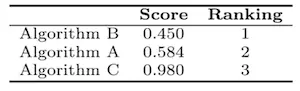
These MSE values would be mapped to the scores (and the corresponding ranking) presented in Table 2. Therefore, Algorithm B would be considered outperforming Algorithm A and Algorithm C.

Table 2: The aggregated score obtained for three competing algorithms A – C, together with the corresponding ranking. Algorithm B is the winner.

Leaderboard

The submitted entries will be ranked based on the metric as outlined above.

To reduce the probability of over-fitting to the test set, the participants will see their results obtained over a subset of the entire test set, referred to as the validation set (V). Note that, in this case, the MSE value obtained by the baseline (“trivial”) solution returning the average value of each parameter will be calculated for the validation set too.

When the challenge closes, the final ranking will be re-computed based on the entire test set ($\psi$), including 1154 test examples. This may lead to changes in the final ranking positions, since the score on the validation set – being a subset of 50% test examples – may differ from the score obtained over the entire test set.

Getting Started

To help you get started with the challenge, we have prepared a Jupyter notebook (Starter Pack) to guide you through the data I/O, visualization, prediction using a baseline algorithm, and creating a valid submission. Please find the starter pack including the Jupyter notebook in this GitHub repository.